دانلود رایگان مقاله رگرسیون غیر پارامتری در R

چکیده

      در مدل های رگرسیون پارامتری سنتی، شکل عملکرد مدل قبل از  تناسب مدل با  دادهَ ها مشخص شده است  و هدف برآوردکردن پارامترهای مدل می باشد. در مقابل، رگرسیون غیر پارامتری، هدف برآورد عملکرد رگرسیون بطورمستقیم بدون مشخص کردن شکل آن به روش صریح می باشد. فاکس و وایزبرگ (2011) در  ضمیمه مقاله، ما توصیف می کنیم چگونه چند نوع مدل رگرسیون غیر پارامتری در R  متناسب  شود، شامل صاف کننده طرح مجزا، که یک پیشگویی واحد وجود دارد؛ مدل های رگرسیون چندگانه؛ مدل های رگرسیون افزایشی؛ و مدل های غير پارامتر-رگرسيون کلی که مشابه مدل های خطی تعميم يافته می باشد.

1 مدل های رگرسیون غیر پارامتری

      مدل رگرسیون غیر خطی سنتی (در ضمیمه در رگرسیون غیرخطی توصیف شد) که  ø یک بردار پارامترهای برآورد شده و x یک بردار پیش بینی کننده است؛ اشتباهات به طور عادی و به طور مستقل با میانگین 0 و واریانس ثابت σ فرض  و توزیع می شود. تابع)  ø m(x,مربوط به مقدار میانگین پاسخ y به پیش بینی کننده ها می باشد، که از قبل مشخص شده است، همانطور که در مدل رگرسیون خطی است.

2.  برآورد

      روش های متعددی برای تخمین مدل های رگرسیون غیر پارامتری وجود دارد که ما دو مورد توصیف خواهیم کرد: رگرسیون چندجمله ای محلی و اسپیلین های صاف. با توجه به پیاده سازی  این روش ها در R، شرمندگی زیادی به همراه خواهد داشت: 

• رگرسيون چندجمله ای محلی با استفاده از تابع استاندارد لس R  انجام می شود (به صورت محلی با صاف کننده طرح مجزا وزنی، برای پرونده ساده رگرسیون) و لس (رگرسیون محلی، بصورت کلی تر) 

• برآورد رگراسیون-ساده نوار-صاف توسط تابع استاندارد R  نوار-صاف انجام می شود

• رگراسیون کلی غیرپارامتریک با برآورد احتمالی محلی (که رگراسیون محلی مورد خاصی برای مدلهایی با خطای عادی هستند) که در بسته لاک فیت (تناسب محلی) (لورد 1999) اجرا می شود که برآورد چگالی را انجام می دهد.  

• مدل های افزایشی عمومی ممکن است متناسب با عملکرد گروهی هستی  و تیبشیرانی (1990) )در بسته گروهی باشد)، که از صاف کننده اسپلین یا محلول رگرسیون محلی استفاده می کند. عملکرد gam در بسته بندی وود mgcv (2000، 2001، 2006)  بخشی از توزیع استاندارد R است، همچنین این کلاس از مدل ها با استفاده از صاف کننده اسپلین و ویژگی های انتخاب اتوماتیک پارامترهای صاف کننده نیز استفاده می شود )نام بسته روش مورد استفاده برای انتخاب پارامترهای هموار حاصل می شود: چندین اعتبارسنجی متقابل تعمیم یافته).

• چندین بسته R دیگر برای رگرسیون غیر پارامتری وجود دارد شامل  بومان وآزالینی (1997 (بسته sm  نرم کننده که رگرسیون محلی و برآورد احتمال محلی را انجام می دهند و همچنین شامل امکانات برای تخمین چگالی غیر پارامتری می باشد؛ و گو (2000)   بسته sm  )اسپلاین صاف کردن عمومی) که متناسب با مدل های رگرسیون تعمیم یافته و  رگراسیون اسپلاین صاف کننده مختلف می باشد.  این  لیست جامع نیست!

2.1 رگرسیون چندجمله ای محلی

2.1.1 رگرسیون ساده

      روال است که h  تنظیم می شود تا اینکه هر رگرسیون محلی شامل یک مقدار ثابت s داده ها می باشد.سپس، S دامنه صاف کننده رگرسیون محلی نامیده می شود.  طول بزرگتر، نتيجه  نرمتر در مقابل، ترتیب بزرگتر رگرسیون های محلی می باشد، لذا دامنه و مرتبه رگرسیون های محلی راحت تر است تا به صورت یک طرفه به فروش برسد.

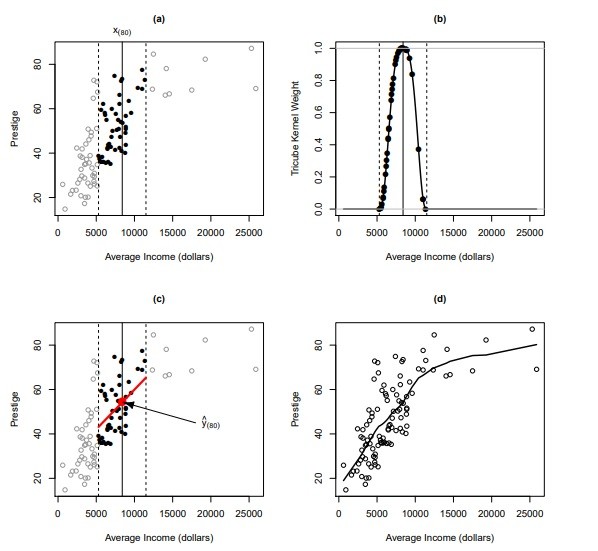
       روند تناسب رگرسیون محلی در شکل 1 نشان داده شده است، با استفاده اطلاعات معتبر شغلی کانادایی در متن فصل 2 بیان شده است. ما رگرسیون اعتبار را در درآمد، در ابتدا تمرکز بر مشاهده با 80 مقدار بزرگ درآمد، x (80)، در شکل 1 توسط خط عمودی جامد نشان داده شده است .   

• یک پنجره شامل  نزدیکترین 50 –همسایگان x  (80) ( (یعنی برای فاصله S = 50 = 102 = 1 = 2) در شکل 1a نشان داده شده است. 

• وزن tricube برای مشاهدات در این همسایگی در شکل 1b نشان داده شده است.

2.1.2 رگرسیون چندگانه

       تعیین درجه = 1 متناسب با  رگرسیون خطی محلی؛ به طور پیش فرض درجه = 2 (یعنی، رگرسیون های محلی درجه دوم است). برای درک کردن طیف وسیعی از استدلال برای تابع لس ، لس مشورت کنید؟  خروجی خلاصه شامل انحراف معیار از باقیمانده های مدل زیر و برآورد تعداد معادل پارامترها (یا درجه آزادی) است که توسط مدل | در این مورد، حدود هشت پارامتر استفاده می شود. در مقابل، مدل رگرسیون خطی استاندارد  از سه پارامتر (ثابت و دو دامنه) استفاده  خواهد کرد.

       همانطور که در رگرسیون ساده غیر پارامتری، برآوردهای پارامتری وجود ندارد: برای درک نتیجه رگرسیون، ما باید سطح رگرسیون نصب شده را به صورت گرافیکی بررسی کنیم، همانطور که در شکل 2 توسط دستورات  زیر R تولید می شود.

        ما از تابع شبکه گسترش استفاده می کنیم تا کادر داده ای حاوی ترکیبی از مقادیر دو پیش بینی کننده، درآمد و آموزش می باشد؛ برای هر پیش بینی کننده، ما مقادیر 25 را به طور مساوی در امتداد دامنه متغیر تقسیم می کنیم. سپس، مقادیر متناسب مربوط به سطح رگرسیون،  با پیش بینی محاسبه  می شوند.  این مقادیر پیش بینی شده به ماتریس 25 تا 25 تغییر یافته است که برای تابع persp همراه با مقادیر پیش بینی کننده (inc و ed)  تصویب می شود  که برای تولید سطح رگرسیون استفاده می شود. استدلال theta و phi  به persp  جهت گیری طرح را کنترل می کند؛  کنترل طول نسبی محور z را گسترش می دهد و سایه ، سطح هاشور خورده  نمودار را کنترل  می کند برای جزئیات بیشتر به ?persp مراجعه کنید

Abstract

       In traditional parametric regression models, the functional form of the model is specified before the model is fit to data, and the object is to estimate the parameters of the model. In nonparametric regression, in contrast, the object is to estimate the regression function directly without specifying its form explicitly. In this appendix to Fox and Weisberg (2011), we describe how to fit several kinds of nonparametric-regression models in R, including scatterplot smoothers, where there is a single predictor; models for multiple regression; additive regression models; and generalized nonparametric-regression models that are analogs to generalized linear models.

1 Nonparametric

      Regression Models The traditional nonlinear regression model (described in the Appendix on nonlinear regression) where is a vector of parameters to be estimated, and x is a vector of predictors; the errors  are assumed to be normally and independently distributed with mean 0 and constant variance  2 . The function ø m(x,, relating the average value of the response  to the predictors, is specified in advance, as it is in a linear regression model. 

2 Estimation

       There are several approaches to estimating nonparametric regression models, of which we will describe two: local polynomial regression and smoothing splines. With respect to implementation of these methods in R, there is an embarrassment of riches: ˆ Local polynomial regression is performed by the standard R functions lowess (locally weighted scatterplot smoother, for the simple-regression case) and loess (local regression, more generally). ˆ Simple-regression smoothing-spline estimation is performed by the standard R function smooth.spline. ˆ Generalized nonparametric regression by local likelihood estimation (of which local regression is a special case for models with normal errors) is implemented in the locfit (local fitting) package (Loader, 1999), which also performs density estimation. 2 ˆ Generalized additive models may be fit with Hastie and Tibshirani’s (1990) gam function (in the gam package), which uses spline or local-regression smoothers. The gam function in Wood’s (2000, 2001, 2006) mgcv package, which is part of the standard R distribution, also fits this class of models using spline smoothers, and features automatic selection of smoothing parameters. (The name of the package comes from the method employed to pick the smoothing parameters: multiple generalized cross-validation.) ˆ There are several other R package for nonparametric regression, including Bowman and Azzalini’s (1997) sm (smoothing) package, which performs local-regression and local-likelihood estimation, and which also includes facilities for nonparametric density estimation; and Gu’s (2000) gss (general smoothing splines) package, which fits various smoothing-spline regression and generalized regression models. This is not an exhaustive list!

2.1 Local Polynomial Regression

2.1.1 Simple Regression

      It is typical to adjust ℎ so that each local regression includes a fixed proportion of the data; then,  is called the span of the local-regression smoother. The larger the span, the smoother the result; in contrast, the larger the order of the local regressions 푝, the more flexible the smooth, so the span and the order of the local regressions can be traded off against one-another.

      The process of fitting a local regression is illustrated in Figure 1, using the Canadian occupationalprestige data introduced in Chapter 2 of the text. We examine the regression of prestige on income, focusing initially on the observation with the 80th largest income value, 푥(80), represented in Figure 1 by the vertical solid line.2

ˆ A window including the 50 nearest -neighbors of (80) (i.e., for span  = 50/102 ≈ 1/2) is shown in Figure 1a.

ˆ The tricube weights for observations in this neighborhood appear in Figure 1b.

2.1.2 Multiple Regression

       Specifying degree=1 fits locally linear regressions; the default is degree=2 (i.e., locally quadratic regressions). To see the full range of arguments for the loess function, consult ?loess. The summary output includes the standard deviation of the residuals under the model and an estimate of the equivalent number of parameters (or degrees of freedom) employed by the model — in this case, about eight parameters. In contrast, a standard linear regression model would have employed three parameters (the constant and two slopes).

       As in nonparametric simple regression, there are no parameters estimates: To see the result of the regression, we have to examine the fitted regression surface graphically, as in Figure 2, produced by the following R commands.

        We employ the expand.grid function to create a data frame containing combinations of values of the two predictors, income and education; for each predictor, we take 25 values, evenly spaced along the range of the variable. Then, corresponding fitted values on the regression surface are computed by predict. These predicted values are reshaped into a 25 by 25 matrix, which is passed to the persp function, along with the values of the predictors (inc and ed) used to generate the regression surface. The arguments theta and phi to persp control the orientation of the plot; expand controls the relative length of the 푧 axis; and shade controls the shading of the plotted surface. See ?persp for details

چکیده

1 مدل های رگرسیون غیر پارامتری

2.  برآورد

2.1 رگرسیون چندجمله ای محلی

2.2 اسپلاین های صاف

2.3  انتخاب پارامتر صاف

2.4 رگرسیون غیر پارامتری افزودنی

3. رگرسیون غیر پارامتر کلی

4. منابع و خواندن مکمل

Abstract

1 Nonparametric Regression Models

2 Estimation

2.1 Local Polynomial Regression

2.2 Smoothing Splines

2.3 Selecting the Smoothing Parameter

2.4 Additive Nonparametric Regression

3 Generalized Nonparametric Regression

4 Complementary Reading and References

References